Representing Text To Vector

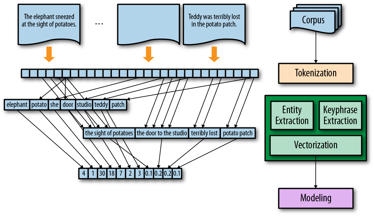
Any Deep Learning model trains on a numeric features present in N dimensional space. In order to perform a language modeling on text, a text must be transformed into its vector representation so that machine learning or deep learning models can be used on the text data. This process of converting a text to a vector is called the Vectorization. In this post, I will discuss about the most widely used vectorization techiniques and mathematical intuition behind all those techniques. So lets dive in!

Text Vectorization Techniques

Some of the most commonly used text vectorization techniques are-

• Bag Of Words
• TF-IDF 
• W2Vec
• Glove

Out of all these techniques, W2Vec and Glove are used widely due to their ability to take into account the semantic meaning of words while converting text into vectors.

Bag Of Words

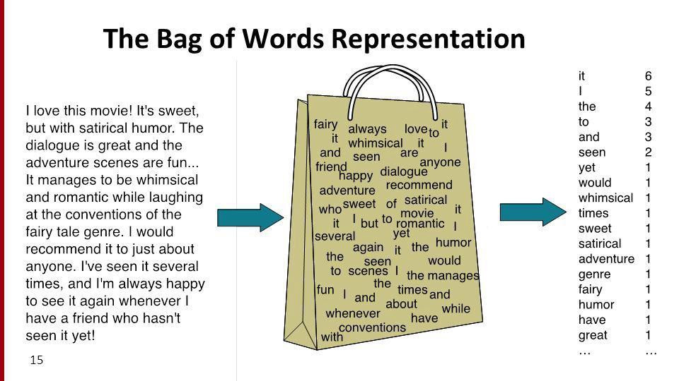
Bag Of Words(BOW) is one of the simplest techniques to convert a text into a vector. A bag-of-words is a representation of text that describes the occurrence of words in a document. It involves two things:

• A vocabulary of known words.
• A measure of the presence of known words.

It is called a bag because the order of the words is not preserved and it is only concerned if a word is present in the corpus or not. A simple intuition behind this representation is that two text corpora are similar if they have the same words in them. Let’s take a simple example and try to understand how it works.

Step 1- Data Collection

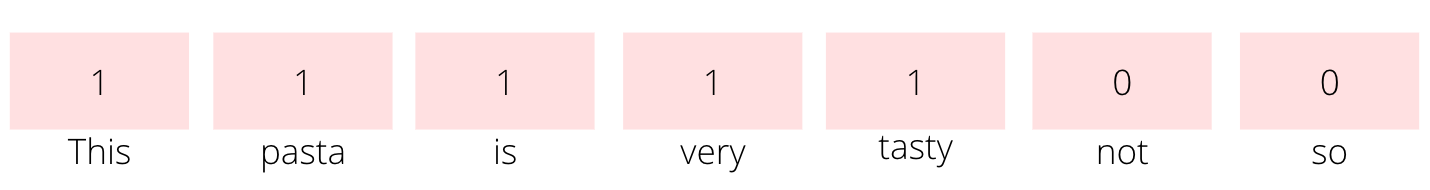
• This pasta is very tasty.
• This pasta is not so tasty.

Consider the above two lines as two text reviews from the single text corpus. Unique words in the above reviews are

Step 2- Creating a vocabulary

• This
• pasta
• is
• very
• tasty
• not
• so

These are the 7 unique words in the whole corpus of 11 words.

Step 3- Create Document Vectors

Bag Of words Vector For First Sentence -

Bag Of words Vector For Second Sentence -

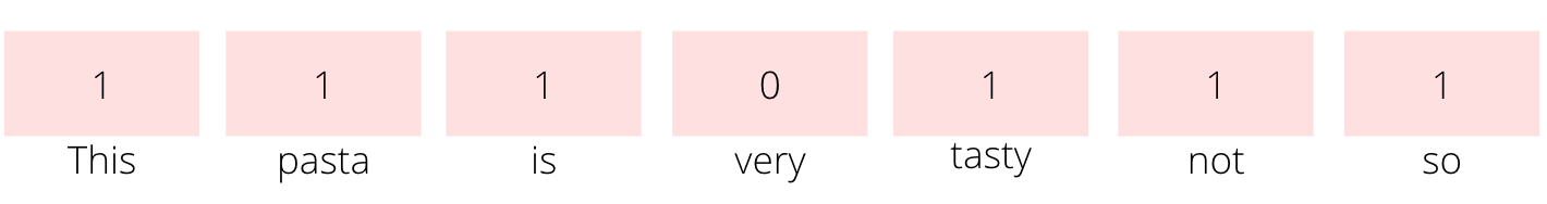
While creating the BOW vector it will consider each of the words in the vocabulary and count the number of times that word appeared in the whole text corpus. This count is used as a vector representation for each word in the text corpus.

Advantages of Bag Of Words

• Simple to understand and implement.

Disadvantages of Bag Of Words

• Curse of Dimensionality- If the unique words in the corpus are too high and there are many words with low frequency then it will lead to a sparse vector representation of BOW. Sparse vector is difficult for a model to compute as well as to interpret. So the performance metrics of a model would be low since the model won’t be able to interpret the features properly.

• Vocabulary- The vocabulary of the BOW needs to be created carefully. The text corpus should be preprocessed with some of the techniques like removing stopwords/punctuations, stemming, lemmatization, converting to lower case, etc. This will significantly reduce the sparsity and also help the model to interpret the vector in a better manner.

• Not Considering The Meaning- The biggest drawback of BOW is ignoring the meaning of the words in the corpus. The meaning of the words brings intuition to the whole sentence. BOW is not taking into account this while vectorizing. This is one of the biggest disadvantages of a BOW words vectorization.

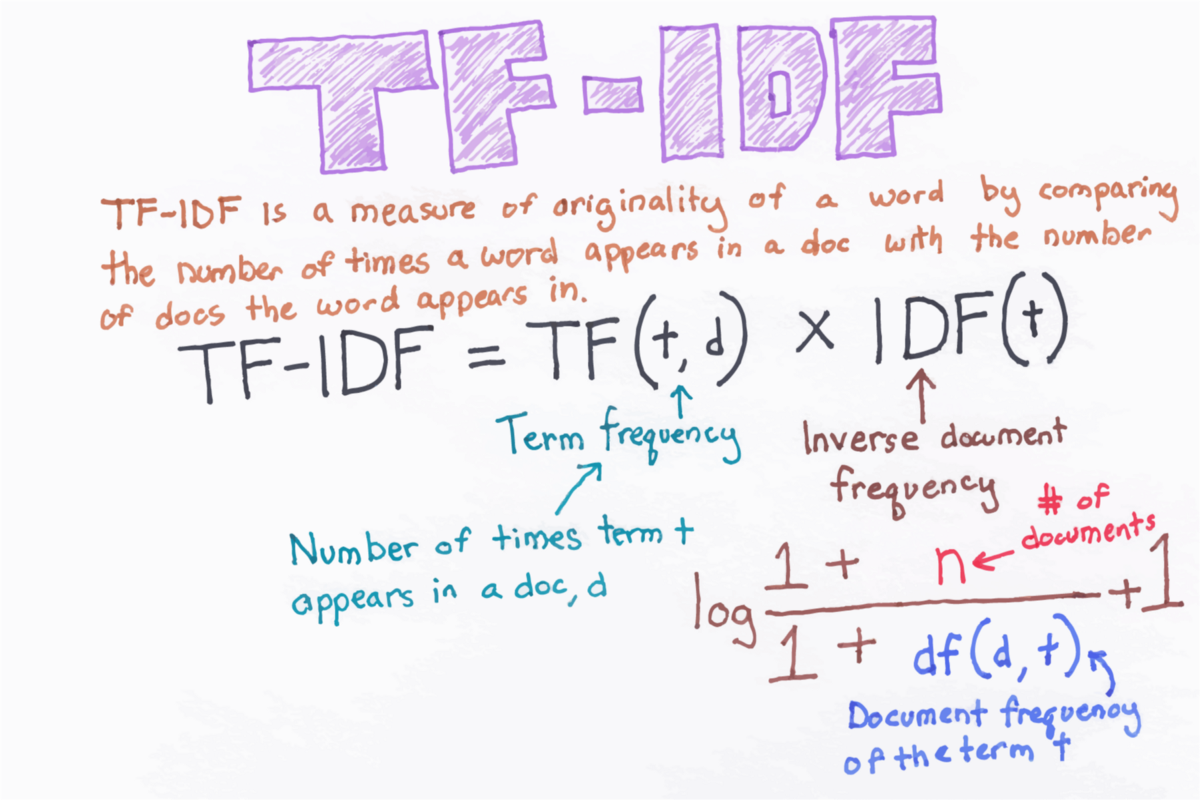
TF-IDF (Term Frequency- Inverse Document Frequency)

TF-IDF is a measure of the originality of a word by comparing the number of times the word appears in a document with the number of documents the word appears in. Term frequency (TF) is how often a word appears in a document, divided by total number of words present in the document. The Inverse Document Frequency (IDF) is a measure of how much information the word provides, i.e. if it’s common or rare across all documents. It is the logarithmically scaled fraction of the total number of documents by the number of documents containing the term. Above Equation of TF-IDF represents a simplified TF-IDF formula.

Need Of Log Term In IDF Formula

In simple as well as modified TF-IDF formula there is a log term in the IDF formula. To understand why log term is needed let’s look at the formula of IDF without considering the log term (I am considering only a simplified version of the IDF here). Without the log term formula of IDF would look like N/df. In this N is the total number of documents and df is the total number of documents in which term is present. Lets assume there were 100000 documents and the term for which IDF is being calculated is present in only 10 documents then the IDF term would be 100000/10 = 10000. The term frequency in TFIDF would be too low as compared to the IDF value calculated above. So if TF-IDF is calculated without the log term then IDF part of the formula will dominate the overall value of the TF-IDF. Instead of that if we use log in the IDF then this value of IDF will be log(10000)= 4 which is significantly lower than the one without log term.

Consider the following document which has two sentences in it

d1: “Hey man! How are you? I thought you moved to New York. How come you are here in LA?”

d2: “How on earth can someone be that stupid?”

Let’s calculate the TF-IDF vector for the word “How” using the simple TF-IDF formula (Assuming all the punctuation are removed and preprocessing is done before calculating the TF-IDF vector)

TF(“How”,d1) = 2 (“How” appeared two times in d1) / 19(Total number of terms in d1)

TF(“How”,d2) = 1 (“How” appeared once in d2)/ 8(Total number of terms in d2 )

IDF(“How”,D) = log(2/2) = 0

TF-IDF(“How”,d1,D) = 0.10526315789 * 0 = 0

TF-IDF(“How”,d2,D) = 0.125 * 0 = 0

One can see that TF-IDF is turning out to be 0. This will definitely make the importance of word which is occurring in every document irrelevant. So with the modified formula of TF-IDF as shown in the figure below,

The purpose of adding the +1 is to accomplish one of the two objectives

a) To avoid divide by zero error as when a term appears in no documents

b) To set a lower bound to avoid a term being given a zero weight just because it appeared in all documents.

According to modified TF-IDF formula-

IDF(“How”,D) = (log(1+2/1+2)) +1= 1

TF-IDF(“How”,d1,D) = 0.10526315789 * 1= 0.10526315789

TF-IDF(“How”,d2,D) = 0.125 * 1= 0.125

Advantages of using TFIDF Vector 

• Easy to compute

• You have some basic metric to extract the most descriptive terms in a document

• You can easily compute the similarity between 2 documents using it

Disadvantages of using TFIDF Vector 

• TF-IDF is based on the bag-of-words (BoW) model, therefore it does not capture position in text, semantics, co-occurrences in different documents, etc.

• For this reason, TF-IDF is only useful as a lexical level feature

• Cannot capture semantics (e.g. as compared to topic models, word embeddings)

W2Vec (Word To Vector)

Word2Vec is one of the most powerful techniques in converting a text to a vector. This technique actually takes into consideration the semantic meaning of the words unlike the earlier techniques like Bag Of Words or TF-IDF. It is almost the state of the art method. Intuitively Word2Vec looks at the neighborhood of the target word to predict the target word. One of the best advantages of the Word2Vec model is that it gives the dense vector as an output, unlike the previous techniques.

Word2Vec is a shallow two-layered network, which is trained to reconstruct the linguistic context of the words. It takes a large corpus of words as an input and converts it to a vector of the size of hundreds of dimensions(typically 100 to 300 dimensions). These word vectors are positioned in such a manner that word vectors of the word having similar contexts are located in close proximity and those which have different contexts are set apart in the vector space. Word2Vec is a computationally efficient predictive model for learning word embeddings from raw text.

CBOW (Continuous Bag Of words)

CBOW is a W2Vec model which will predict the target word given the context of the target word.

Sentence: The cheetah ran very fast while hunting the deer.

In this sentence, considering cheetah as a target word, the context words would be “The(c1) ran(c2) very(c3) fast(c4) while(c5) chasing(c6) the(c7) deer(c8)”

Let’s assume we have,

1. The V = vocabulary or dictionary of words and v = Length/Size of the Vocabulary.
2. Using one hot encoding of each word. This will represent each word as a one-hot encoded vector of size v.

Let’s assume we have a huge text corpus and we have created the dataset of the target word and its corresponding context words.

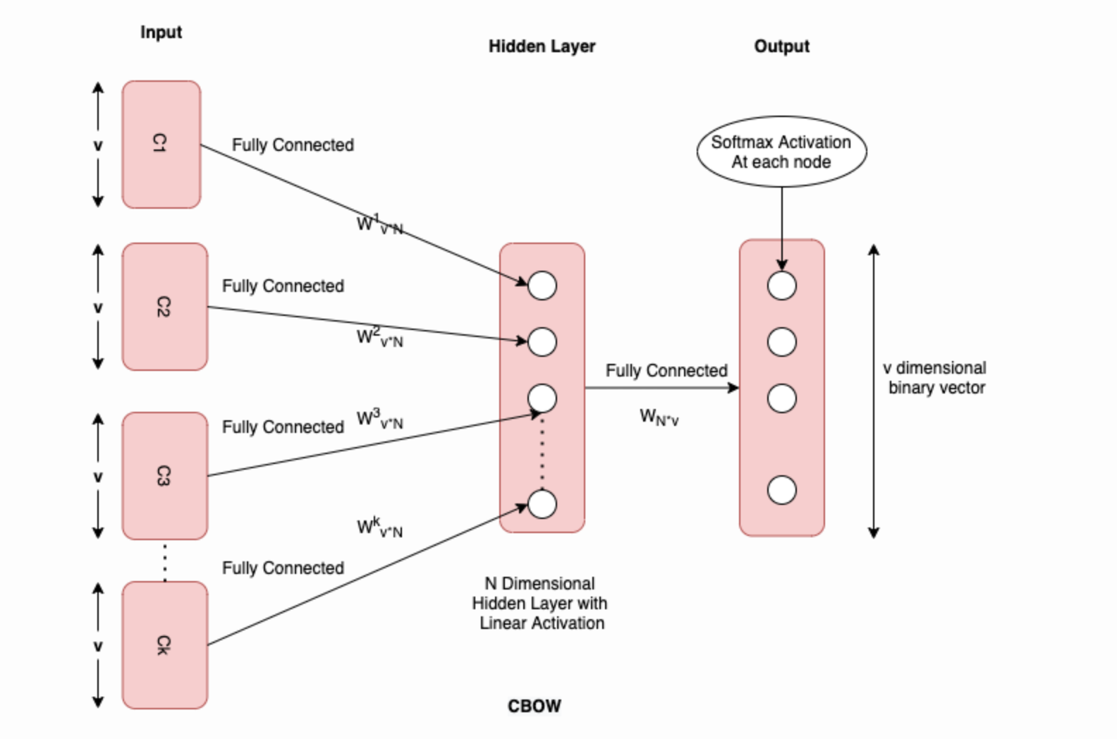
This CBOW is a very simple two-layered neural network and if trained on the dataset which we created, at the output this model will return N * v vector. This N * v vector can be used for vectorization. So given a word W_i we will get corresponding V_i. This corresponding V_i will have a whole vector representation of the size of N dimensions.

Skip-Gram

Skip-Gram predicts surrounding context words from the given target words (inverse of CBOW). Statistically, skip-gram treats each context-target pair as a new observation, and this tends to do better when we have larger datasets.

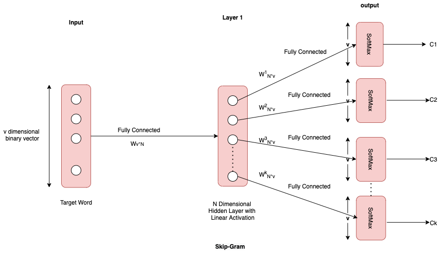
In this Skip-Gram, the target word is provided as an input and the Context vector is the output. In the case of SkipGram W_v*N matrix can be used to get the words.

Advantages of CBOW - 

• Faster than Skip-Gram
• Better for frequently occurring words.

Advantages of Skip-Gram - 

• Can work with a smaller amount of data
• Well for infrequent words

Problem with training the CBOW / SkipGram

If you think about this Skip-Gram solves much harder problem since it is predicts the whole context given just a target word. Whereas in the case of CBOW whole context is given and it just predicts the target word. It’s like filling the blanks problem. But since Skip-Gram solves the much harder problem it works well on many general cases. K is the total number of context words taken into consideration for each target word. If k increases then more context is seen by CBOW and more context will be predicted by Skip-Gram.

There is one major problem in CBOW and SkipGram-

Lets look at number of weights to be trained- 

Number of weights = (K+1) (N * v)

Assume N = 200, k=5, V=10k It will be 12 million weights. This will be a huge computation for any compute. It will take nearly forever to train these networks. So how to optimize this?

Word2Vec Optimization -

We saw that both CBOW and Skip-Gram training will be extremely exhaustive for any compute device. So there are two concepts that are used to train these models efficiently.

Hierarchical Softmax 

If one takes a look at the SkipGram or CBOW connections they both use multiple softmax functions. Computations of these softmax functions are bit exhaustive. So core idea of the hierarchical softmax is to replace these v -softmax functions with something which is computationally less expensive. Softmax activation is trying to solve V class classification. 

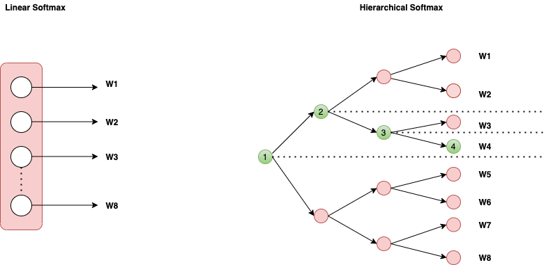
In the case of linear softmax function, for each word in a sentence, one softmax is needed and softmax calculations are computationally expensive. In the above example since we have 8 words, there will be 8 softmax functions. In case of hierarchical softmax, we place 8 words at the leaf node of the binary tree. Hierarchical softmax uses a binary tree to represent all words in the vocabulary. The words themselves are leaves in the tree. For each leaf, there exists a unique path from the root to the leaf, and this path is used to estimate the probability of the word represented by the leaf. This probability is defined as the probability of a random walk starting from the root ending at the leaf in question.

The main advantage is that instead of evaluating v output nodes in the neural network to obtain the probability distribution, it is needed to evaluate only about log₂(v) words. Typically a binary Huffman tree is used, as it assigns short codes to the frequent words which result in fast training.

Negative Sampling 

Negative Sampling is simply the idea that we only update a sample of output words per iteration. The target output word should be kept in the sample and it will get updated, and we add to this a few (non-target) words as negative samples. “A probabilistic distribution is needed for the sampling process, and it can be arbitrarily chosen… One can determine a good distribution empirically.” Each word is discarded with a probability of P(wi) where P(wi ) is,

f(w_i) is the frequency of word w_i and t is a chosen threshold, typically around 10^-5.

Since the negative sampling and the hierarchical softmax are used in the Word2Vec model, it trains much faster and can be used as a vectorization technique with the semantic meaning consideration.

Adavantages Of Word2Vec

• The idea is very intuitive, which transforms the unlabled raw corpus into labeled data (by mapping the target word to its context word), and learns the representation of words in a classification task.
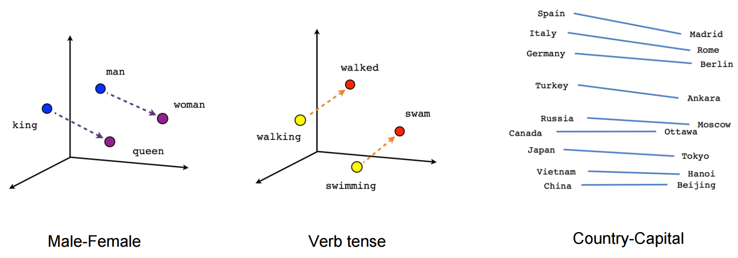
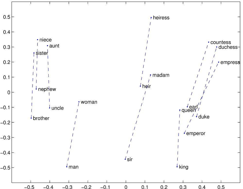
• The mapping between the target word to its context word implicitly embeds the sub-linear relationship into the vector space of words, so that relationships like “king:man as queen:woman” can be infered by word vectors.
• Easy to understand and implement

Disadvantages:

• The sub-linear relationships are not explicitly defined. There is little theoretical support behind such characteristic.
• The model could be very difficult to train if use the softmax function, since the number of categories is too large (the size of vocabulary). Though approxination algorithms like negative sampling (NEG) and hierarchical softmax (HS) are proposed to address the issue, other problems happen. For example, the word vectors by NEG are not distributed uniformally, they are located within a cone in the vector space hence the vector space is not sufficiently utilized.

Glove (Global Vectors For Word Representation)

The Word2Vec doesn’t consider the statistical information of word co-occurrence. This was an inspiration for developing Global Vectors for word representation(Glove). Glove combines the benefits of the Word2Vec SkipGram model in analogy tasks with the benefits of matrix factorization methods that can exploit global statistical information.

Glove algorithm

The GloVe algorithm consists of following steps:

1. Collect word co-occurence statistics in a form of word co-ocurrence matrix X. Each element X_ij of such matrix represents how often word i appears in context of word j. Usually we scan our corpus in the following manner: for each term we look for context terms within some area defined by a window_size before the term and a window_size after the term. Also we give less weight for more distant words, usually using this formula: decay = 1/offset

2. Define soft constraints for each word pair:

   

3. Define a cost function

   

   Here f is a weighting function which help us to prevent learning only from extremely common word pairs. The GloVe authors choose the following function:

   

Advantages:

• The goal of Glove is very straightforward, i.e., to enforce the word vectors to capture sub-linear relationships in the vector space. Thus, it proves to perform better than Word2vec in the word analogoy tasks.
• Glove adds some more practical meaning into word vectors by considering the relationships between word pair and word pair rather than word and word.
• Glove gives lower weight for highly frequent word pairs so as to prevent the meaningless stop words like “the”, “an” will not dominate the training progress.

Disadvantages:

• The model is trained on the co-occurrence matrix of words, which takes a lot of memory for storage. Especially, if you change the hyper-parameters related to the co-occurrence matrix, you have to reconstruct the matrix again, which is very time-consuming.

Conclusion

Out of the four techniques of vectorization, Word2Vec and Glove outperforms BOW and TF-IDF in almost all the cases due to their ability to take semantic meaning into consideration. Even with Word2Vec and Glove vectorizers some challenges still remain, like how to learn the representation for out-of-vocabulary words. how to separate some opposite word pairs like “good” or “bad” which are located in the same vector space nearby.

I tried to explain these vectorization techniques since most people treat this as a blackbox for converting the text to vectors. If you have any questions/suggestions feel free to reach out to me on LinkedIn.

Reference 

• GloVe: Global Vectors for Word Representation

• Word2Vec

• Amazing Power Of Word Vectors