Understanding probability is crucial in machine learning as it aids in handling uncertainty with incomplete data…

Table Of Content -

Introduction
Population and Sample
Gaussian Distribution
Skewness
Kurtosis
Standard Normal Variate
Kernel Density Estimation
Central Limit Theorem
Quantile Quantile Plots
Bernoulli Distribution
Chebyshew Inequality
Log Normal Distribution
Power Law Distribution

Introduction -

Probability is all about handling the uncertainty. Uncertainty involves making decisions based on incomplete information and this is how the whole world operates. Probability is the field of mathematics that gives tools to quantify the uncertanty of the events and reason in principled manner. Machine learning is all about building a predictive model by using uncertain data. There are three main reasons which causes uncertainty in the machine learning which are noisy data, incomplete coverage of problem domain, imperfect models. These all uncertainties can be managed by using tools of probabilty. Some of the aspects in Machine Learning where probability is used are -

Classification models must predict a probability of class membership.
Algorithms are designed using probability (e.g. Naive Bayes).
Learning algorithms will make decisions using probability (e.g. information gain).
Sub-fields of study are built on probability (e.g. Bayesian networks).
Algorithms are trained under probability frameworks (e.g. maximum likelihood).
Models are fit using probabilistic loss functions (e.g. log loss and cross entropy).
Model hyperparameters are configured with probability (e.g. Bayesian optimization).
Probabilistic measures are used to evaluate model skill (e.g. brier score, ROC).

This is the reason why a profound knowledge of probability can be a game changer to understand the machine learning models in depth. So there are lots of thing to cover in this blog so lets dive in with some simple concepts -

Population And Sample-

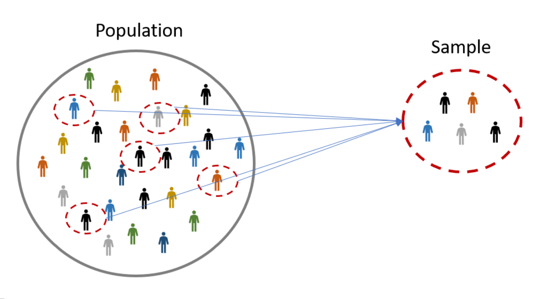
A population is set of similar items or events which are of interest to certain experiment whereas a statistical sample is a set of items selected from the population. For example, there are ~7 Billion people on earth and the experiment is supposed to be conducted to calculate average height of humans on earth. So the population for this experiment would be 7 Billion, but carrying out an experiment on such a large scale is practically impossible. So we take the sample out of this population. Lets say like 5 Million people from all around the globe. So based on this sampled data a predictive model can be built to predict an average height of humans on earth. So to put these concepts simply, we can say that sampled data is a subset of the population and we can say that Sample < Population.

Gaussian Distribution / Normal Distribution-

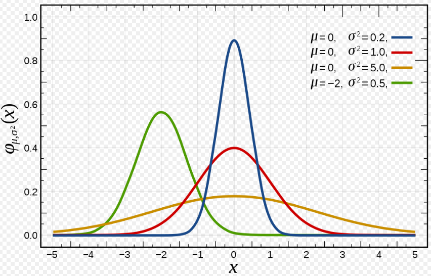
This is one of the most widely used distribution in the field of Machine Learning. The reason why this distribution plays important role in ML is because lots and lots of things in the real world follow this bell curve-like distribution. Eg. Distribution of weights of people in the world of the same age range (let’s consider for people of age 25, Very few people will have a weight lower than 35 kgs and Very few will have a weight above 120kg and many people will have the weight near to the value of let’s say 60–90). The mean of the distribution is 0 so there are many values that belong to mean 0 but as you go away from the mean value the value of the distribution will go on decreasing.

The formula for Probability Density Function(PDF) of a normal distribution is,

Here sigma σ is nothing but the standard deviation and σ² is the variance. μ is the mean.

You can observe that as the value of variance increase the curve gets flatter and widespread. Whereas you can observe that the pdf value is maximum at the mean value.
Normal Distribution has a symmetric PDF.
As X value moves away from μ. Pdf decreases exponentially.

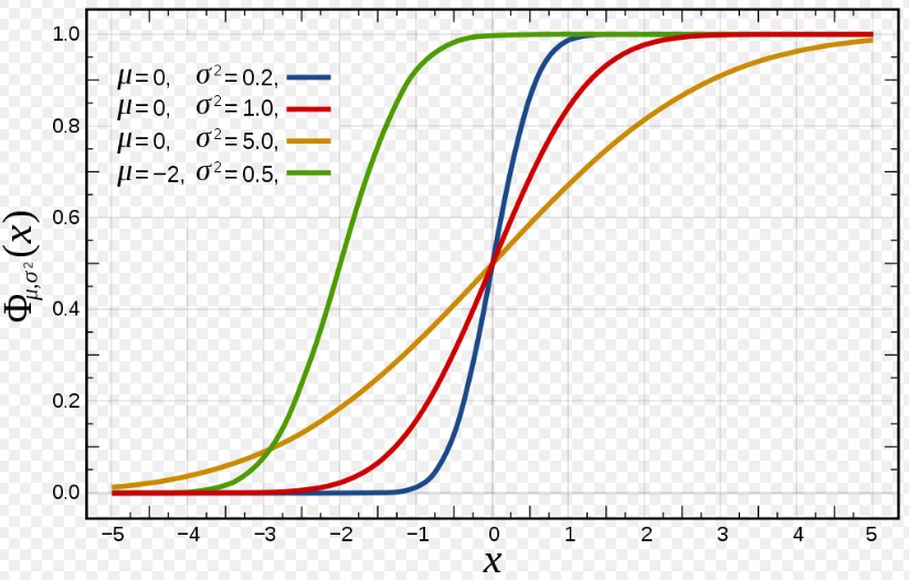
If you take a look at the CDF of a gaussian distribution you can notice that as the variance is low the CDF line gets closer to the μ and as variance decreases the slope of the CDF becomes less steep.

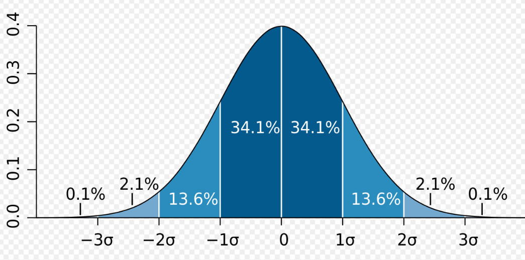
Let’s consider an example to understand the bell curve. Let’s say our distribution is a normal distribution such that X~(μ,σ²)=X~(0,4). We can say that 50% of the values lie on the left side and 50% of the values on the right side of the bell curve. The best part of the bell curve is that we can tell how many values of a sample lie in between the range between the corresponding standard deviation values. For eg. Here as the variance is 4, so the standard deviation is 2. Since std deviation is 2 we can say that between -σ and +σ we will have 68.2% of the values and between -2σ and +2σ value we will have 95% values of the sample.

Skewness-

Skewness is a measure of asymmetry of pdf.

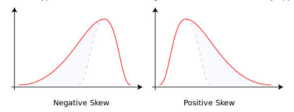
Here x_bar is the sample mean and s is the sample standard deviation, m3 is a sample third central moment. Skewness can be used to approximate probabilities and quantiles of distributions.

Kurtosis-

Kurtosis tells us about the tailedness of a distribution. It tells us how heavily the tails of a distribution differed from the tails of a normal distribution. In other words, kurtosis identifies whether the tails of a given distribution contain extreme values.

It is a good measure of detecting if there are outliers in the dataset or not.
A larger value of kurtosis indicates a serious outlier problem which is a good indication for the researchers to choose an alternative statistical model.
The excess kurtosis is defined as kurtosis minus 3.

Standard Normal Variate-

It is the distribution that occurs when a normal random variable has a mean of zero and a standard deviation of one. The normal random variable of a standard normal distribution is called a standard score or a z score. Every normal random variable X can be transformed into a z score via the following equation: z = (X - μ) / σ.

where X is a normal random variable, μ is the mean, and σ is the standard deviation. It is an extremely helpful way to get rid of the problem of difference in the scales used while measuring. It brings all the values in the range of 0 to 1 so that we can compare the variable values easily. This is just like the standardization of a variable.

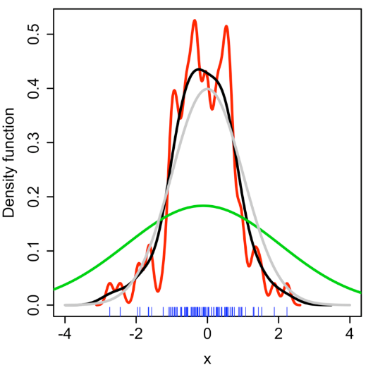
Kernel Density Estimation-

It is a non-parametric way to estimate the pdf of a random variable. Kernel density estimation is a fundamental data smoothing problem where inferences about the population are made, based on a finite data sample.

Variance in this case is called bandwidth. If we take bandwidth value too large then we get wide pdf, if bandwidth value is too small then we get the jagged estimation of a curve. For a smooth curved approximation, bandwidth must be chosen with proper care.

Sampling Distribution-

Let’s say that we have a distribution of variable X which is not necessarily a gaussian, So now let’s say we take n samples from that population, Lets call those S1, S2,…, Sn(Assume the size of each sample<population size). For each sample, we calculate the mean of that sample, and let’s call these x1, x2, x3,…, xn (such that x1,x2,…xn are sample means of each sample S1, S2,…, Sn). Now, x1,x2,x3,…, xn will also have a distribution of their own? So the distribution of xi’s is called the sample distribution of sample means. steps-

Take S1, S2, S3,…, Sn samples out of the population.
Calculate means of each of the samples x1,x2,x3,…, xn
And the distribution of x1,x2,…., xn will be called the sampling distribution of sample means.

References -

https://machinelearningmastery.com/probability-for-machine-learning/